Image inpainting with wavelets

import pywt
import numpy as np
import matplotlib.pyplot as plt
from context import samplers as samplers
from context import utils as utils


def clamp(im,vmin=0,vmax=1):
    return np.minimum(np.maximum(im,vmin),vmax)

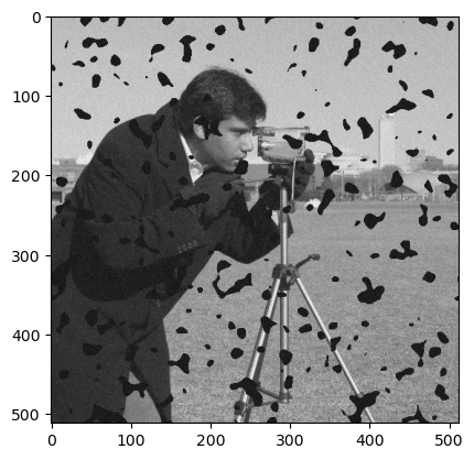
Display \(f =\Phi u + w\) where \(u\) is the camera image and \(s\) is some random Gaussian noise.

from skimage.util import random_noise
from skimage.transform import rescale
import matplotlib.pyplot as plt
from numpy.fft import ifft2,fft2

# load an image
cam = pywt.data.camera()/255
p1,p2 = cam.shape



#Define an inpainting operator
s = 5
h = utils.GaussianFilter_2d(s,p1,p2)
Phi = lambda x: np.real(ifft2(fft2(x)*fft2(h)));
Phi_s = lambda x: np.real(ifft2(fft2(x)*np.conjugate(fft2(h))))

#inpainting
mask = np.random.rand(p1,p2) #random mask
mask = np.abs(ifft2(fft2(mask)*fft2(h)))>0.48 #patchy mask
Phi = lambda x: mask*x
Phi_s = lambda x: mask*x

#observation
b = Phi(cam)
sigma = .001;
b = random_noise(b,mode='gaussian',var=sigma,clip=False) # add noise

plt.imshow(b, cmap="gray")
plt.savefig('results/observation.pdf', bbox_inches='tight')

plt.show()

We will consider the regularisation

\[R_\alpha(f) := \mathrm{argmin}_u \frac12 \| \Phi u - f\|^2 + \alpha\|DW u\|_1\]

where \(W\) is the discrete wavelet transform and \(D\) is a diagonal weighting matrix. Note that since \(W^* = W^{-1}\), we can rewrite this as \(R_\alpha(f) = W^* D^{-1} z_\alpha\) where

\[z_\alpha := \mathrm{argmin}_z \frac12 \| A z - f\|^2 + \alpha\|z\|_1.\]

where \(A:= \Phi\circ W^* \circ D^{-1}\).

#define the operator A
L =int(np.log2(p2))
py_W, py_Ws, scaling_vec = utils.getWaveletTransforms_2D(p1,p2,
                                                         wavelet_type = "haar",
                                                         level = L,weight= 1) #.6

#define forward and adjoint operator
# Phi o W^{-1} o D^{-1}
A = lambda coeffs: Phi(py_Ws(scaling_vec*coeffs))

# D^{-1} o W o Phi
As = lambda im: scaling_vec*py_W(Phi_s(im))

lam = 1.5*.5**6 #regularizatio
lam = 0.005
lam = 0.1
# lam = 0.0001
# lam = 0.0005



print(lam)
mfunc = lambda x: .5* np.linalg.norm(A(x)-b,ord='fro')**2 + lam*np.linalg.norm(x,ord=1)
prox = lambda x, tau: np.maximum(np.abs(x)-tau, 0)*np.sign(x)

0.1

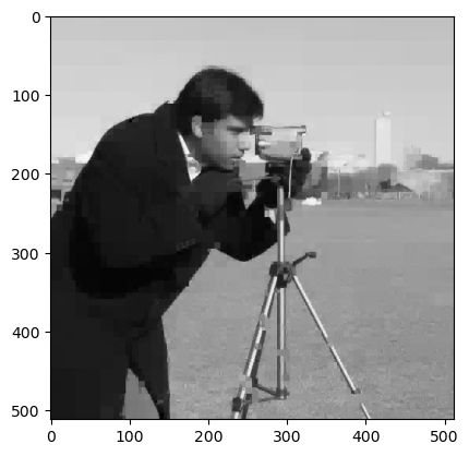
run restarted fista to compute the mode and display

tau = 1/2 #stepsize
nIter =500
dG = lambda x: As(A(x) - b)
proxF = lambda x,tau: prox(x,tau*lam)
xinit = As(b)

#run restarted fista
x_mode,fval = utils.rFISTA(proxF, dG, tau, xinit,nIter,mfunc)


plt.imshow(clamp(py_Ws(scaling_vec*x_mode)), cmap="gray",vmin=0,vmax=1)
plt.savefig('results/mode.pdf', bbox_inches='tight')

plt.show()

# plt.semilogy(fval-min(fval))

p = len(xinit)
x = np.random.randn(p,)
nm_est = np.linalg.norm(As(A(x)))/np.linalg.norm(x)
print('estimated norm of |A^* A|', nm_est)

estimated norm of |A^* A| 0.948257530921056

Lf = 1 #*np.linalg.norm(h)*len(cam)
# Lf = 0.2
gamma = 1/Lf/50 #1/(np.linalg.norm(h)*len(cam)) #moreau reg parameter for prox-l1
tau = gamma/(5*(gamma*Lf + 1)) #stepsize
print('tau:', tau, 'gamma:', gamma)

lam = .1 #l1 regularization parameter
beta = 5 #inverse temperature

p = p1*p2


grad_F = lambda x:  dG(x) + (x - prox(x,lam*gamma))/gamma
Iterate = lambda x: samplers.one_step_langevin(x,p, grad_F, tau,beta=beta)
xinit = np.random.randn(p,)


n = 300
burn_in = 10000

Iterate_uv = lambda x: samplers.one_step_hadamard(x, p,dG, tau, lam,beta=beta)
uvinit = np.random.randn(2*p,)*0.001
uvinit[:len(xinit)] = np.abs(uvinit[:len(xinit)])
samples_uv = samplers.generate_samples_stride(Iterate_uv, uvinit, n, stride=20, burn_in=burn_in)
print('uv sampler done\n')

samples = samplers.generate_samples_stride(Iterate, xinit, n,stride=20, burn_in=burn_in)
print('prox_l1 sampler done\n')

tau: 0.00392156862745098 gamma: 0.02
uv sampler done

prox_l1 sampler done

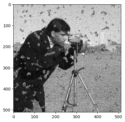
Display mean image for uv

samples_x_uv = samples_uv[:,:p]*samples_uv[:,p:]
im_average = py_Ws(scaling_vec*np.mean(samples_x_uv, axis=0))

plt.imshow(clamp(im_average.reshape(p1,p2)) ,cmap='gray', vmin=0, vmax=1)
plt.savefig('results/uv_mean.pdf', bbox_inches='tight')

Display mean image for prox-langevin

im_prox_average = py_Ws(scaling_vec*np.mean(samples,axis=0))
plt.imshow(clamp(im_prox_average), cmap='gray', vmin=0, vmax=1)
plt.savefig('results/prox_mean.pdf', bbox_inches='tight')

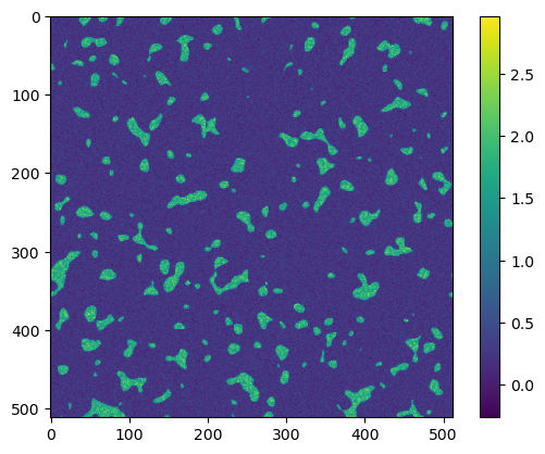
Show the difference between the 95 and 5 quantiles

n = samples_x_uv.shape[0]
signal_uv= [py_Ws(scaling_vec*samples_x_uv[i,:]) for i in range(n)]
signal_uv = np.array(signal_uv)

n = samples.shape[0]
signal_prox= [py_Ws(scaling_vec*samples[i,:]) for i in range(n)]
signal_prox = np.array(signal_prox)

lower_bound_uv = np.percentile(signal_uv, 5, axis=0)
upper_bound_uv = np.percentile(signal_uv, 95, axis=0)

lower_bound_prox = np.percentile(signal_prox, 5, axis=0)
upper_bound_prox = np.percentile(signal_prox, 95, axis=0)

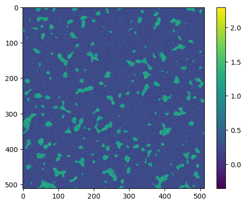
plt.imshow(np.log(upper_bound_uv-lower_bound_uv).reshape(p1,p2))#,vmin=0,vmax=-2)
plt.colorbar()
plt.savefig('results/uv_percentile.pdf', bbox_inches='tight')

plt.imshow(np.log(upper_bound_prox-lower_bound_prox).reshape(p1,p2))#,vmin=0,vmax=-2)
plt.colorbar()
plt.savefig('results/prox_percentile.pdf', bbox_inches='tight')

display video for hadamard

%matplotlib inline

import matplotlib.pyplot as plt
import numpy as np

import matplotlib.animation as animation

fig, ax = plt.subplots()

K = 1
ims = []
for i in range(n//K):

    im = ax.imshow((signal_uv[i*K]),cmap='gray' ,animated=True, vmin=0, vmax=1)
    if i == 0:
        ax.imshow((signal_uv[i] ),cmap='gray', vmin=0, vmax=1)  # show an initial one first
    ims.append([im])

ani = animation.ArtistAnimation(fig, ims, interval=50, blit=True,
                                repeat_delay=1000)


f = r"uv.gif"
writergif = animation.PillowWriter(fps=30)
ani.save(f, writer=writergif)

from IPython.display import HTML
HTML(ani.to_jshtml())

Animation size has reached 21145662 bytes, exceeding the limit of 20971520.0. If you're sure you want a larger animation embedded, set the animation.embed_limit rc parameter to a larger value (in MB). This and further frames will be dropped.

Once Loop Reflect

## display video for prox-l1

%matplotlib inline

import matplotlib.pyplot as plt
import numpy as np

import matplotlib.animation as animation

fig, ax = plt.subplots()

K = 1
ims = []
for i in range(n//K):

    im = ax.imshow((signal_prox[i*K]),cmap='gray', animated=True,vmin=0,vmax=1)
    if i == 0:
        ax.imshow((signal_prox[i]),cmap='gray',vmin=0,vmax=1)  # show an initial one first
    ims.append([im])

ani = animation.ArtistAnimation(fig, ims, interval=50, blit=True,
                                repeat_delay=1000)

f = r"prox.gif"
writergif = animation.PillowWriter(fps=30)
ani.save(f, writer=writergif)

from IPython.display import HTML
HTML(ani.to_jshtml())

Animation size has reached 21237014 bytes, exceeding the limit of 20971520.0. If you're sure you want a larger animation embedded, set the animation.embed_limit rc parameter to a larger value (in MB). This and further frames will be dropped.

Once Loop Reflect

check the ESS

import arviz as az

idata_uv = az.convert_to_inference_data(np.expand_dims(signal_uv, 0))
ess_uv = az.ess(idata_uv)

idata = az.convert_to_inference_data(np.expand_dims(signal_prox, 0))
ess = az.ess(idata)

plt.plot(ess_uv['x'].values.reshape(-1),'g', alpha=0.5,label='Hadamard')
plt.plot(ess['x'].values.reshape(-1),'r',alpha=0.5, label='Prox-l1')

plt.legend()
plt.savefig('results/ess.pdf', bbox_inches='tight')

np.min(ess['x'].values),np.min(ess_uv['x'].values)

(1.3226521711517507, 1.3285242420266064)

plt.imshow(np.log(ess['x'].values),vmin=0.3,vmax=4.4)
plt.colorbar()
plt.savefig('results/prox_ess.pdf', bbox_inches='tight')

plt.imshow(np.log(ess_uv['x'].values),vmin=0.3,vmax=4.4)
plt.colorbar()
plt.savefig('results/uv_ess.pdf', bbox_inches='tight')

plt.imshow(b, cmap="gray")
plt.savefig('results/observation.pdf', bbox_inches='tight')