from context import samplers as samplers

import numpy as np


def soft(x,tau):
    return np.sign(x)*np.maximum(np.abs(x)-tau,0)


def make_prox_kernel(tau, grad, lam, gamma, p, beta=1):
    grad_F = lambda x:  grad(x) + (x - soft(x,lam*gamma))/gamma

    def step(z):
        return samplers.one_step_langevin(z, p, grad_F, tau,beta)
    return step

def make_hadamard_kernel(tau, grad, lam, p,beta=1):
    def step(z):
        return samplers.one_step_hadamard(z, p, grad, tau, lam,beta)
    return step

def project_hadamard(z, p):
    return z[:p] * z[p:]

Visualize paths in 2D

import matplotlib.pyplot as plt

np.random.seed(10)


p = 2
lam = 2
beta= 1.

# smooth part: G(x) = 1/2 ||x||^2
grad = lambda x: x

A = np.array([[1.0, 0.0],
              [0.0, .1]])   # second direction weak
y = np.array([1.0, 1.0])


Lf = np.linalg.norm(A.T@A, 2)
gamma= 1/Lf/10
# tau = gamma/5/(Lf*gamma+1)
tau = 1/10/Lf


def grad(x):
    return A.T @ (A @ x - y)

def fval(x):
    r = A @ x - y
    return 0.5 * np.dot(r, r)

# initial points
x0 = np.array([2.0, -2.0])
z0 = np.concatenate([np.ones(p), x0])  # (u,v)

# kernels
prox_step = make_prox_kernel(tau, grad, lam, gamma, p,beta)
had_step = make_hadamard_kernel(tau, grad, lam, p,beta)

# simulate
T = 2000
traj_prox = [x0]
traj_hadam = [project_hadamard(z0, p)]

x = x0.copy()
z = z0.copy()

for _ in range(T):
    x = prox_step(x)
    z = had_step(z)
    traj_prox.append(x.copy())
    traj_hadam.append(project_hadamard(z, p))

traj_prox = np.array(traj_prox)
traj_hadam = np.array(traj_hadam)

# grid and contour
xx, yy = np.meshgrid(np.linspace(-5,5,200), np.linspace(-8,7,200))
xx, yy = np.meshgrid(np.linspace(-3,3,200), np.linspace(-3,3,200))

Z = 0.5*(A[0,0] *xx + A[0,1]*yy - y[0])**2 + 0.5*(A[1,0] *xx + A[1,1]*yy - y[1])**2 + lam*(np.abs(xx)+np.abs(yy))

from scipy.stats import gaussian_kde
from matplotlib.collections import LineCollection

def plot_trajectory(traj):
    # Color line by local visit density
    xy = traj.T  # shape (2, n)
    density = gaussian_kde(xy)(xy)

    points = traj.reshape(-1, 1, 2)
    segments = np.concatenate([points[:-1], points[1:]], axis=1)
    lc = LineCollection(segments, cmap='viridis', linewidth=0.8, zorder=1,alpha=0.6)
    lc.set_array(density)

    plt.gca().add_collection(lc)


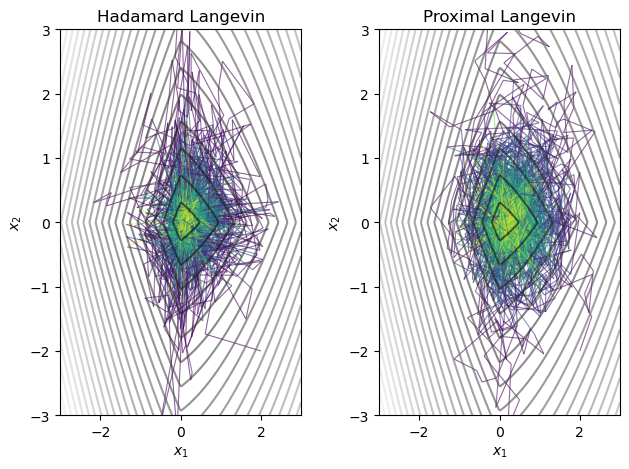
plt.subplot(1, 2, 1)
plt.contour(xx, yy, -Z, levels=30, cmap='gray_r',  zorder=2, alpha=.6)

plot_trajectory(traj_hadam)
plt.xlabel("$x_1$")
plt.ylabel("$x_2$")

plt.title("Hadamard Langevin")
# plt.show()


# Gibbs
plt.subplot(1,2,2)
plt.contour(xx, yy, -Z, levels=30, cmap='gray_r', zorder=2, alpha=.6)

plot_trajectory(traj_prox)

plt.title("Proximal Langevin")
plt.xlabel("$x_1$")
plt.ylabel("$x_2$")

plt.tight_layout(w_pad=2)
plt.show()

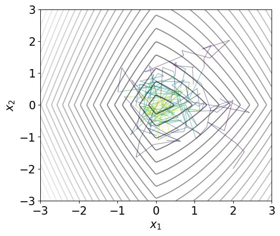
plt.contour(xx, yy, -Z, levels=30, cmap='gray_r',  zorder=2, alpha=.6)

plot_trajectory(traj_prox)

plt.xlabel("$x_1$", fontsize=16)
plt.ylabel("$x_2$", fontsize=16)
plt.tick_params(axis='x', labelsize=16)
plt.tick_params(axis='y', labelsize=16)
plt.gcf().set_size_inches(6, 5)

plt.savefig(str(T) +'prox10.pdf', bbox_inches='tight')

Visualize (u,v) or (x,eta) for case \(d=1\)

from scipy.stats import invgauss

def sample_eta_given_x(x, lam, beta):
    eta = np.zeros_like(x)
    for j in range(len(x)):
        mu = abs(1./(beta*lam*np.abs(x[j]) + 1e-8))  # avoid division by 0
        eta[j] = 1 / invgauss.rvs(mu=mu, scale=(lam*beta)**2)
    return eta

def hadamard_to_x_eta(z, p, beta):
    u = z[:p]
    v = z[p:]
    x = u * v
    eta = (u**2) / beta / lam
    return x, eta

import matplotlib.pyplot as plt

p = 1
lam = 1.5
beta= 1

gamma= 1/6
tau = gamma/5/(gamma+1)

# smooth part: G(x) = 1/2 ||x||^2
grad = lambda x: 2*(x-1)
def fval(x):
    return  (x-1)**2


# initial points
x0 = np.array([-1.0])
z0 = np.concatenate([np.ones(p), x0])  # (u,v)

# kernels
prox_step = make_prox_kernel(tau, grad, lam, gamma, p)
had_step = make_hadamard_kernel(tau, grad, lam, p)

#generate trajectories
T = 10000
# store trajectories
traj_uv = []
traj_x_eta = []
traj_x_eta_hadam = []

x = x0.copy()
z = z0.copy()

for _ in range(T):
    # proximal step
    x = prox_step(x)
    eta = sample_eta_given_x(x, lam, beta)

    # hadamard step
    z = had_step(z)
    u, v = z[:p], z[p:]

    #convert hadamard to x,eta
    x_uv, eta_uv = hadamard_to_x_eta(z, p, beta)
    traj_x_eta_hadam.append([x_uv[0], eta_uv[0]])

    # store only first coordinate (clean 2D plot)
    traj_uv.append([u[0], v[0]])
    traj_x_eta.append([x[0], eta[0]])

traj_uv = np.array(traj_uv)
traj_x_eta = np.array(traj_x_eta)
traj_x_eta_hadam = np.array(traj_x_eta_hadam)

# contours
uu, vv = np.meshgrid(np.linspace(0.001,3,200), np.linspace(-1.5,2.5,200))
X = uu * vv
Z_uv = beta*(fval(X)  +0.5* lam*uu**2 + 0.5* lam*vv**2) - np.log(uu)


xx, ee = np.meshgrid(np.linspace(-1,3,200), np.linspace(.00001,7,200))
Z_xe = beta*fval(xx) + 0.5*(xx**2 / ee) +0.5* lam**2*beta**2 * ee + np.log(np.sqrt(ee))

from scipy.stats import gaussian_kde
from matplotlib.collections import LineCollection

def scatter_trajectory(traj):
    xy = traj.T  # shape (2, n)
    density = gaussian_kde(xy)(xy)

    plt.scatter(
        traj[:,0],
        traj[:,1],
        c=density,
        cmap='viridis',
        s=5,
        alpha=0.2,
        zorder=1
    )


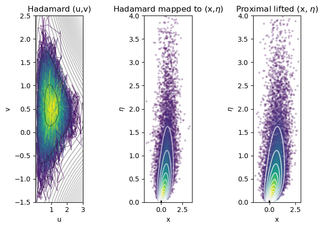
# 1. trajectories of u,v from hadamard-langevin

plt.subplot(1, 3, 1)
plt.contour(uu, vv, ( -Z_uv), levels=50, cmap='gray_r', alpha=0.3)

plot_trajectory(traj_uv)

plt.xlabel("u")
plt.ylabel("v")
plt.title("Hadamard (u,v)")


# 2. scatter x-eta from hadamard-langevin
plt.subplot(1, 3, 2)
plt.contour(xx, ee, np.exp(-Z_xe), levels=400, cmap='gray_r',  zorder=2, alpha=0.6)
scatter_trajectory(traj_x_eta_hadam)

plt.title("Hadamard mapped to (x,$\eta$)")
plt.xlabel("x")
plt.ylabel("$\eta$")
plt.ylim([0,4])


# 3. scatter x-eta from prox-langevin
plt.subplot(1,3,3)

# background contour
plt.contour(xx, ee, np.exp(-Z_xe), levels=400, cmap='gray_r', alpha=.7, zorder=2)
scatter_trajectory(traj_x_eta)

# plt.colorbar(label="density")
plt.title("Proximal lifted (x, $\eta$)")
plt.xlabel("x")
plt.ylabel("$\eta$")
plt.ylim([0,4])


plt.tight_layout(w_pad=5)

plt.show()